6.1 Stars
6.1.1 Stellar masses
Stellar masses are computed by multiplying a mass-to-light
ratio M∕L with a luminosity L. While the uncertainties on
L depend on the quality of the data, the estimate over
M∕L and its associated uncertainties depend mostly on the
care taken with SED fitting. It is a good idea to search fora reference band that minimizes the effects of M∕L
variations due to stellar populations (age, metallicity,
chemical abundances) and due to dust absorption.
While the common notion that the NIR (e.g. the H
band at 1.65 μm) is close to ideal is correct in some
cases, problems can arise because of thermally pulsing
asymptotic giant branch stars (discussed in section 2.1.3) if
young ages (<2 Gyr) are well represented in the SED.
That reliable M∕L from SED fitting cannot be dispensed
with is evident when looking at IRAC 3.6μm data of
nearby galaxies, where star formation regions are evidently
prominent.
Stellar Mass Maps of Resolved Galaxies
In the work of Zibetti, Charlot, and Rix (2009) a
“data-cube” approach is introduced to investigate the
SEDs of nearby, resolved galaxies, aimed at preserving the
maximum spatially-resolved information. One feature of
the approach is that it allows to compare “global”
quantities, which are notoriously difficult to determine,
with the integral over the local quantities, a useful test of
how meaningful global quantities can be. A large part of
the effort concentrated on developing a reliable method
to obtain stellar surface mass density maps from a
minimum set of broad-band observations. This method
relies on Bayesian inference, as discussed in Section
4.5.
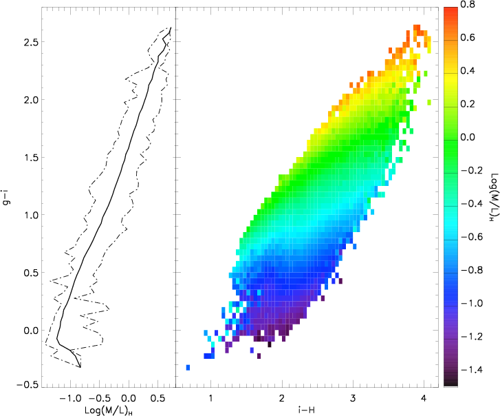
The effective mass-to-light ratio correlates with optical /
near-infrared colors (e.g., Bell and de Jong 2001), so M∕L
can be expressed as a function of color(s). A better
estimate is obtained if M∕L is mapped as a function of two
colors, instead of one. The colors adopted are g - i
and i - H. Their large wavelength separation allows
to robustly describe the shape of the SED over the
entire optical-near-infrared range, in a way that as
insensitive as possible to photometric and modeling
uncertainties.
To study the dependence of M∕L on (g-i,i-H) the
authors use a Monte Carlo library of 50,000 models created
from the 2007 version of BC03, which include also dust
in different amounts and spatial distributions.. The
(g-i,i-H) space is binned in cells of 0.05 mag ×
0.05 mag and marginalized over M∕L in each cell. The
median is chosen as the fiducial M∕L at each position of
the color-color space. A look-up table is created to
derive M∕LH as a function of (g-i,i-H). Figure 23
illustrates that the information in the second color
improves the M/L determinations systematically by
±0.3–0.4 dex.
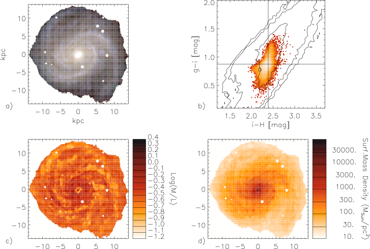
The method described above is applied to each pixel of
the image of a galaxy, where “pixel” implies the pixel
that results after matching the images in the three
bands to a common resolution. In order to provide
sensible results, it is crucial that color measurements do
not exceed 0.1 mag errors, which requires S/N~20.
The results for M 100 (NGC 4321) are displayed in
Figure 24.
An important result appears from the comparison
between total stellar mass as obtained by integrating the
stellar mass surface density maps (Figure 24d) and the one
obtained using global colors to estimate the “average”
M∕L ratio to be multiplied by L(H). This second method,
the one commonly adopted in extragalactic studies,
agrees within ~10% of the mass map integral only
when the color distribution is quite homogeneous,
i.e., for early type galaxies. When substantial color
inhomogeneities and especially heavily obscured regions are
present within a galaxy, using global colors and fluxes
can lead to underestimates of the actual stellar mass
of a galaxy by up to 60%. This can be understood
if dust-obscured regions can contribute a significant
amount of mass but are heavily under-represented in
the global color, which is flux weighted and hence
biased toward the brightest (and bluest) parts of the
galaxy. While the pixel-by-pixel M∕L gives the correct
mass weight to these obscured regions, the globally
computed M∕L severely underestimates their mass
contribution.
Stellar mass functions
One of the holy grails of current observational efforts in
galaxy evolution studies is a consistent picture of the
build-up of stellar mass over the age of the universe. An
important constraint on this is the stellar mass function, or
its integral, the stellar mass density. A comprehensive
discussion of these results would warrant a review of its
own. Suffice it here to point out that not only the local
mass function has been measured with great precision
(e.g. Bell et al. 2003a), but these results have also been
extended to redshifts of 1 (Pozzetti et al. 2007; Bundy
et al. 2006). At redshifts above 1.2 an observed-frame
optical selection corresponds to a rest-frame UV selection,
subject to large biases. These therefore have to be
circumvented by a K-band selection (e.g. Cirasuolo
et al. 2007) or, better, by a selection at 3.6μm (Arnouts
et al. 2007; Ilbert et al. 2010, e.g.). For observational
and conceptual reasons (detailed in Sections 4.5.2
and 4.6), determining stellar masses and therefore
mass function at redshifts higher than z=2 is very
difficult. Most authors thus prefer to restrict themselves
to luminosity functions instead (see e.g. Cirasuolo
et al. 2010, for just one very recent example), thus
leaving the burden of transforming luminosities to stellar
masses to the interpreting model (but see e.g. Kajisawa
et al. 2009).
Stellar masses of high redshift galaxies
Many authors have used some kind of Bayesian
inference-based method (Section 4.5) to determine stellar
masses for high redshift galaxies (e.g. Sawicki and
Yee 1998; Papovich, Dickinson, and Ferguson 2001; Förster
Schreiber et al. 2004). There is good hope that these
mass estimates are reasonably good (Drory, Bender,
and Hopp 2004), despite important caveats on the
methodology that become more important with improving
data quality (see e.g. Section 4.1). A recent result has
been the discovery and study of high redshift galaxies with
high stellar masses and low star formation rates (early type
galaxies, ETGs). In the following we describe only one
”family” of papers, as presented at the workshop, but
see Cimatti (2009) for a review. Massive ETGs are
the first objects to populate the red sequence (see
e.g. Kriek et al. 2008b). Objects in the redshift range 2-3
can be identified by multi-band photometry (e.g. van
Dokkum et al. 2006). For determining the physical
properties however, significant uncertainties are due to
photometric redshift determinations. For example
Kriek et al. (2008) conclude that while stellar masses
are reasonably robust to small errors arising from photometric redshifts, the actual star formation history is
generally very poorly constrained with broad band data
alone.
The obvious next step is thus to analyze these galaxies
with spectroscopy, despite this being an expensive
undertaking in terms of telescope time. When doing this,
Kriek et al. (2008) also go further in blurring the limits
between spectroscopy and photometry by binning
their “low” S/N spectra into bins of 400 Å. While the
information content remains unchanged, this certainly
leads to improvements in presentability and fitting speed.
Kriek et al. (2009a) then show explicitly that provided
enough photons can be assembled through either exposure
time or telescope size, the spectra of galaxies at redshifts
2-3 are amenable to the same kind of analysis as in the
local universe. The upshot of these studies is that
massive, compact ETGs with very little residual star
formation are in place already at redshifts between 2 and
3.
Despite these successes, the study of Muzzin
et al. (2009a,b) confirms that even using spectroscopic
data, model uncertainties mean that SED-derived stellar
masses are affected with uncertainties of factors 2-3 at
these redshifts. For further discussion on stellar mass
determinations the reader is also referred to the review by
de Jong & Bell (in prep.).
6.1.2 Deriving SFHs from spectroscopy
Comparing observations to semi-analytic models
Trager and Somerville (2009) extend the semi-analytic
model of Somerville et al. (2008) to predict the line
absorption strengths (Section 4.2) of the resulting galaxies.
This allows them to use the same analysis tools that would
be used in the analysis of the measured line strengths of an
observed sample of galaxies on objects with known
properties, in particular star formation histories. They
select in particular early type galaxies from the mock
catalogues they produce and compute the index strengths
of the resulting spectra. These index strengths can then be
plotted on the same plots as real data. They come to the
sobering conclusion that while the sample of Trager,
Faber, and Dressler (2008) is of sufficient quality do
do a meaningful comparison, it remains too small.
On the other hand large samples of galaxies, as the
one of Moore et al. (2002), still lack the required
precision.
The archeology of the universe
The database of the SDSS spectra has been used to
derive the SFH of galaxies from their current spectra
(e.g. Heavens et al. 2004, see also Section 4.4), a
procedure sometimes called “unlocking the fossil record” or
simply “astro-archeology”. A recent update on this has
been presented in Tojeiro et al. (2007), who applied
VESPA (see Section 4.4) to the SDSS sample of spectra
and derived a catalogue that was made available to the
community at http://www-wfau.roe.ac.uk/vespa/. It
provides detailed star formation histories and other
parameters for SDSS’s latest data release (DR7) of the
Main Galaxy Sample and the Luminous Red Galaxies
sample. Details of the catalogue, including description,
basic properties and example queries can be found in
(Tojeiro et al. 2009).
Combining spectroscopic and dynamic ages
The use of spectroscopy in combination with dynamical
arguments to understand the evolution of a single
object was presented in Pappalardo et al. (2010). The
galaxy NGC4388 is a member of the Virgo cluster
and sports a huge trail of HI gas (Oosterloo and van
Gorkom 2005). It represent an ideal study case for the
effects of ram stripping on a galaxy moving in the
intra-cluster medium (Vollmer and Huchtmeier 2003). The
stripping age has been estimated to be of order 200
Myr from dynamical arguments. Using VLT/ FORS
spectroscopy of the outer and inner regions of the galaxy
and the STECKMAP program (Ocvirk et al. 2006),
Pappalardo et al. (2010) were able to show that, while the
inner region of the galaxy is of solar metallicity and has
continued forming stars to the present day, the outer
regions of the galaxy have sub-solar metallicity and have
stopped forming stars roughly 200 Myrs ago, in accordance
with the dynamical estimate. Single cases like this
can thus help identify the processes and timescale
associated with shutting down the star formation in
galaxies, one of the most profound changes a galaxy can
experience.
Star formation rates
Star formation rates from SED fitting have been little
used, with most authors preferring to rely on single
tracers (see Section 4.5.3 for a comparison). Walcher
et al. (2008) have used stellar masses and star formation
rates consistently derived from the same SED fit to
compare the predicted evolution of the stellar mass
function to the observed one. The main result is that while
stars form in blue cloud galaxies, most of the growth of the
stellar mass function occurs in quiescent galaxies, in
agreement with studies based on different tracers of star formation (e.g. Bell et al. 2007). From comparison with
merger studies in the same field, Walcher et al. (2008)
conclude that about half of the mass growth on the red
sequence comes from major mergers and half from minor
mergers.
Salim et al. (2007) have compared their SED-fitting
SFRs to SFRs determined from emission lines. They find
that some galaxies with no detected emission lines
nevertheless have substantial SED-based SFRs. They
attribute this result to “recent” star formation, i.e. stars
that formed long enough ago that their emission lines
already vanished, but still recently enough to be revealed
in the galaxy SED. Recent HST imaging in the UV which
clearly shows SF structures seems to confirm this (Salim &
Rich 2010, ApJ submitted).
6.1.3 Identifying and studying outliers
This is an underexplored use of SED fitting, in the opinion
of the authors. One example, objects with differing SFR
measurements from emission lines and SED fitting has
been covered in the last section.
Finding Wolf-Rayet stars
The availability of large databases of spectra, such as
from the SDSS, and of accurate stellar population
model predictions enables the search for rare objects or
systematic deviations that are not predicted by the
model itself. An example of this are Wolf-Rayet stars,
evolved, massive stars with characteristic features. These
have ages between 2 × 10⁶ and 5 × 10⁶ years, and
are thus a transient feature of galaxy spectra. They
are useful as a tracer of recent star formation history
as well as the metallicity of their host galaxies. As
shown in Brinchmann, Kunth, and Durret (2008),
a systematic search in the SDSS database yields a
sample several times larger than previous serendipitous
searches. The essential ingredient of such a search is the
accuracy of the stellar population model that allows an
inversion technique (Section 4.4) to be applied on a
large sample. Indeed, either a smooth correction or
residual features from inaccurate models would severely
impair the identification of the specific features. As
an example Brinchmann, Kunth, and Durret (2008)
show that the use of the Bruzual and Charlot (2003)
models produced a large number of false positives,
while an updated version of the same model using
different stellar spectra (CB09) provides much better
fits.