2.1 Stars

In its simplest sense, a galaxy is a population of stars ranging from numerous, low-luminosity, low-mass stars, to the bright, short-lived, massive OB stars. On closer examination, these stars are distributed in both metallicity content and age ranging from when the galaxy first formed to those newly born. The method of creating a galactic spectrum through the sum of the spectra of its stars is called stellar population synthesis and was pioneered in works by Tinsley (1972), Searle, Sargent, and Bagnuolo (1973) and Larson and Tinsley (1978). A simplification for the modelling of galactic SEDs is that the emitted light can be represented through a sum of spectra of simple stellar populations (SSPs) with different age and element abundances. Here a SSP is an idealized single-age, single-abundance ensemble of stars whose distribution in mass depends on both the initial distribution and the assumed age of the ensemble.

There are two main methods used by current stellar spectrophotometric models to compute the SEDs of SSPs: The first is called ’isochrone synthesis’. It uses the locus of stars with the same age, called an isochrone, in the Hertzsprung-Russel diagram and then integrates the spectra of all stars along the isochrone to compute the total flux. This method was established by Chiosi, Bertelli, and Bressan (1988); Maeder and Meynet (1988) and in particular Charlot and Bruzual (1991) and is currently used by the majority of stellar population models. The second uses the ‘fuel consumption’ approach. One of the problems of the isochrone synthesis method was that isochrones are calculated in discrete steps in time and therefore phases where stellar evolution is more rapid than theses timesteps were not well represented (the most famous example of the last years being the thermally pulsing asymptotic giant branch stars). Models using the fuel consumption theorem circumvent this problem by changing the integration variable above the main sequence turnoff to the stellar fuel, i.e. the amount of hydrogen and helium used in nuclear burning. The fuel is integrated along the evolutionary track. The main idea is that the luminosity of the post-main sequence stars, which are the most luminous, is directly linked to the fuel available to stars at the turnoff mass (for full details, see e.g. Buzzoni 1989; Maraston 1998, 2005). While these methods are fundamentally different in their integration methods, most of the issues discussed here in terms of stellar evolution and stellar libraries apply to both.

2.1.1 Simple stellar populations

The spectrum (flux emitted per unit frequency per unit mass), L_ν, of a SSP of mass M, age t, and metallicity Z is given by the sum of the individual stars:

(1)

In practice the emitted light is dominated by the most massive, luminous stars.

The stellar mass function, ϕ(M)_t,Z, is computed from an initial mass function (IMF, ϕ₀(M)) and stellar evolution, which describes when and which stars will stop contributing to the SSP spectra because they end their lives either as Supernovae or as white dwarfs. The IMF describes the distribution in mass of a putative zero-age main sequence stellar population and is an input parameter of stellar population synthesis models. The IMF is usually limited between a minimum and maximum stellar mass (generally M_min ~ 0.05 - 1.0M⊙; M_max ~ 100 - 150M⊙). Three empirical forms are most commonly used: a simple power-law model (Salpeter 1955; Massey 1998), a broken power-law (Kroupa 2001), or a lognormal form (Chabrier 2001). However whether these forms hold in all conditions and for all redshifts is still an open question (A good coverage of this field can be found in the “IMF@50” proceedings, E. Corbelli, F. Palla, & H. Zinnecker 2005).

The true difficulty of calculating equation 1 lies in the second part, determining the SED (L_ν) of a star of initial mass, M, age, t, and metallicity, Z. This requires; 1) the computation of stellar evolutionary tracks that determine where a star of given stellar parameters (e.g. mass M, age t and abundance Z) lies on the Hertzsprung-Russel diagram or log g - T_eff diagram, to build up the stellar ’isochrone’, and 2) the computation or empirical building of a stellar library of L_ν with full coverage of log g,T_eff, and Z to determine what the resulting spectrum of such a star is.

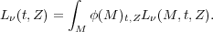
The creation of stellar isochrones requires a large grid of evolutionary tracks, created by modelling the evolution of stars of a given initial mass and metal content. Over the past few decades, much work has gone into providing homogeneous sets of stellar tracks from different groups, e.g. Padova (Marigo and Girardi 2007; Marigo et al. 2008), Geneva (Lejeune and Schaerer 2001), Yale (Demarque et al. 2004), MPA(Weiss and Schlattl 2008), BaSTI (Pietrinferni et al. 2009). For SSP modelling, the models generally run from the start of the main sequence (Zero Age Main Sequence, ZAMS) to some end point of the star, such as a supernova or the asymptotic giant branch (AGB) phase. Originally computed only for a solar metallicity composition and a few stellar masses, sets of homogeneous stellar evolutionary tracks now exist for a wide range of initial masses (from ~ 0.1M⊙ to ~ 120 M⊙; see e.g. Girardi et al. 2000; Meynet and Maeder 2005) and metallicities (~ 0.01 to ~ 4Z_⊙). In most stellar evolutionary modelling it has been assumed that for all stellar masses the elemental composition is the same for a given metallicity, however more recently the evolutionary effects of elemental variations such as α-enhancement (e.g. Salasnich et al. 2000) or individual element variations (e.g. Dotter et al. 2007) have been investigated. However problems still remain in the field, with the different treatments by the different groups still giving distinct evolutionary tracks even with the same inputs, as shown in figure 1.

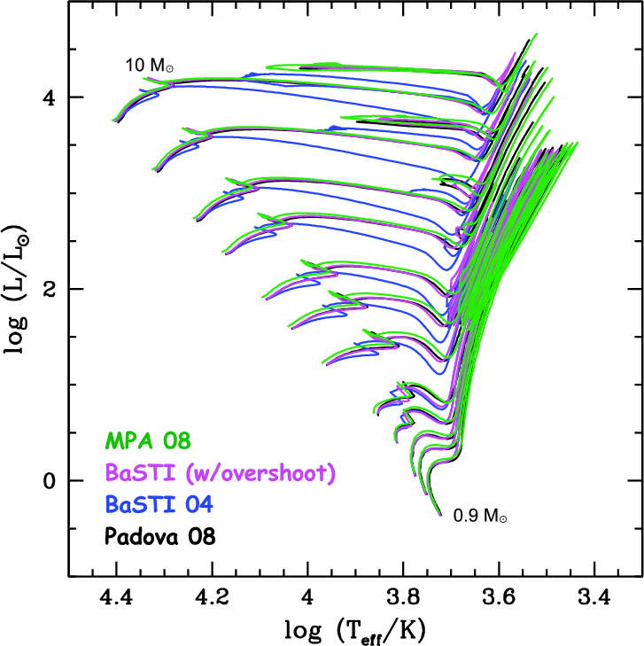
While the evolutionary tracks lead to the generation of an isochrone, to determine a SSP spectrum, a library of stellar spectra is needed, covering the necessary parameter space in log T_eff, log g, metallicity etc. As with the evolutionary tracks, stellar libraries have improved significantly in recent years, with both fully theoretical (e.g. Kurucz 1992; Westera et al. 2002; Smith, Norris, and Crowther 2002; Coelho et al. 2005; Martins et al. 2005; Lançon et al. 2007) and empirical, e.g. STELIB (Le Borgne et al. 2003), MILES (Sánchez-Blázquez et al. 2006; Cenarro et al. 2007), Indo-US (Valdes et al. 2004), ELODIE (Prugniel and Soubiran 2001; Prugniel et al. 2007), HST/NGSL (Gregg et al. 2004) libraries covering much greater parameter spaces and increasing in both spectral and parameter resolution (see figure 2). Unlike the optical, the UV still suffers from incomplete libraries which is specially important for fully exploiting data on high redshift galaxies (see e.g. Pellerin and Finkelstein 2009). The question about which of empirical or theoretical libraries is preferable is a matter of the specific application (for a short review on both sets of libraries and their respective issues, see Coelho 2009). The main benefit of the empirical libraries is that they are based on real stars and thus avoid uncertainties in stellar atmosphere structure or in opacities. On the other hand, due to the observational limits they cover a restricted parameter space biased towards Milky way compositions (see e.g. Cenarro et al. 2007). Additionally, the determination of their fundamental parameters can be difficult for some types of stars and is itself based on stellar models. Conversely theoretical libraries can cover a much larger parameter space and at any chosen resolution (see e.g. Martins et al. 2005). There are still known problems in the comparison between the observed and theoretical stellar spectra (Martins and Coelho 2007). Two specific examples for problems of theoretical models are incomplete line lists (Kurucz 2005), problematic particularly at high spectral resolution, and the modelling of the IR emission (Lançon et al. 2007), which is particularly difficult for stars in the luminosity classes I and II (A. Lançon, talk at workshop). The way forward may be a synthesizing approach, as suggest by Walcher et al. (2009), aimed at using the strengths of both kinds of libraries. As with the evolutionary tracks, most libraries are limited to single compositions for a given metallicity. However recently this also has been changing, with stellar libraries exploring abundance changes such as α-enhancement as well (e.g. Coelho et al. 2007) .

It is not much of an overstatement to say that the magic of stellar population evolutionary synthesis spectrophotometric codes lies in interpolation. Indeed, to go from evolutionary tracks to isochrones (quoting Maeder and Meynet 1988) “the interpolation between evolutionary tracks must be properly based on point of corresponding evolutionary status” (see also Prather 1976), and similarly to go from an isochrone to SSP SED, the correct, often interpolated, spectrum must be found for each mass bin. These stellar population synthesis (SPS) codes, using stellar evolutionary tracks and stellar libraries, then calculate Equation 1. Besides interpolation, the challenge is to create the most homogeneous and most accurate set of input ingredients, interpolating in an appropriate manner when necessary in dependence on the coverage and strengths of these sets. Stellar population models predicting full spectra include; Fioc and Rocca-Volmerange (1997, PEGASE), Bressan, Granato, and Silva (1998, used in GRASIL) and Leitherer et al. (1999) and Vázquez et al. (2007) (both Starburst99), Vazdekis (1999), Schulz et al. (2002), Cerviño, Mas-Hesse, and Kunth (2002), Robert et al. (2003), Bruzual and Charlot (2003, GALAXEV, also commonly referred to as BC03), Le Borgne et al. (2004, PEGASE-HR), Maraston (2005, M05, based on fuel consumption theorem), Lançon et al. (2008), Mollá, García-Vargas, and Bressan (2009). Currently less frequently used are fully theoretical stellar population models such as González Delgado et al. (2005); Coelho et al. (2007). However, as recently shown by Walcher et al. (2009), a combination of semi-empirical and fully theoretical models holds great promise for the future. As a result of the improvements in stellar evolutionary tracks and stellar libraries, as well as the codes themselves, stellar population synthesis models today can recreate broad-band UV to NIR SEDs and high-resolution spectra in the optical remarkably well.

2.1.2 Validation of SSP predictions

As SSP spectra form the basis of all fitting of galaxy SEDs and as the complexities of real galaxies may introduce degeneracies and further uncertainties in the resulting interpretations, it is of primary importance to validate directly the predictions of the stellar population synthesis models for SSPs (see e.g. Bruzual A. 2001). For the impact of uncertainties in the stellar parameters effective temperature, surface gravity, and iron abundance on the final SSPs see Percival and Salaris (2009).

The ideal testbed for such validations are simple stellar populations occurring in nature, i.e. co-eval stellar populations such as globular clusters (GCs), open clusters, and young star clusters. These objects have been used as such for some time (e.g. Renzini and Fusi Pecci 1988; González Delgado and Cid Fernandes 2010), but unfortunately, the exact equivalence between star clusters and SSPs breaks down for a number of reasons:
1) In star clusters, the stellar populations are affected by the dynamical evolution of the cluster, which leads to mass segregation, and evaporation of low-mass stars in GCs and, in young star clusters, the expulsion of gas early in their life time may lead to dissolution (open clusters) or to the loss of a significant number of stars (though see Anders, Lamers, and Baumgardt 2009, for recent work on dealing with this in SSP models).
2) Clusters also contain exotic stars (e.g. blue straggler stars, discussed in the following section) which influence the integrated light of the cluster but are not accounted for by most population synthesis models (though see Xin, Deng, and Han 2007, for a discussion on how to account for these).
3) Finally, star clusters only have a finite number of stars. In a less than 10⁵ M_⊙ star cluster, the number of bright stars is so small, that stochastic fluctuations in the photometric properties of the cluster are common (Barbaro and Bertelli 1977; Lançon and Mouhcine 2000a; Cerviño and Luridiana 2004, 2006; Piskunov et al. 2009).

In the study of individual clusters, most of these problems might be alleviated by concentrating on the most massive specimens (W3, ω Cen, starburst clusters), but these have the tendency to exhibit multiple rather than single (simple) stellar populations (e.g. Lee et al. 1999). Thus, one needs to study star cluster populations for comparison with SSP models and to account for the influence of the stochastic fluctuations on the color-luminosity distribution. Looking the other way around, within a given error box for the observed colors, a complex distribution of possible ages is possible (Fouesneau et al., talk at workshop). While multi-wavelength observations help, they do not completely eliminate the problem.

2.1.3 Current Issues with SSPs

Even though significant improvements in the evolutionary tracks and stellar libraries have been made in the last decade, significant challenges remain, as some parts of stellar evolution are only weakly understood, and hence poorly treated. The most important of these tend to be short lived but bright phases: massive stars, thermally pulsing asymptotic giant branch (TP-AGB) stars, extreme horizontal branch stars (EHB) and blue stragglers.

Massive stars, due to their rapid evolution and short lifetime, prove to be difficult to model and observe at all phases. Additional difficulties arise in that they tend to be buried by the interstellar material that they formed from for a large fraction of their lifetime, and experience high stellar winds (and hence strong mass evolution over their lifetime). Yet massive stars are a vital component of SSP modelling because they are so luminous and can thus dominate a SSP spectrum, and because they give rise to most of the ionizing flux and resulting nebular emission-line contribution. Previous modelling of massive star evolution paid particular attention to the size of the convective core and stellar mass loss, yet recent theory has indicated the significant, if not dominant, role that stellar rotation has on the evolution of these stars (Meynet and Maeder 2005). Vázquez et al. (2007) show in their recent stellar population model that, as rotating stars tend to be bluer and more luminous than in earlier models, even the ionizing spectrum can be significantly altered. These differences have consequences when interpreting the SEDs of young galaxies, such as decreasing the determined mass or star formation rates.

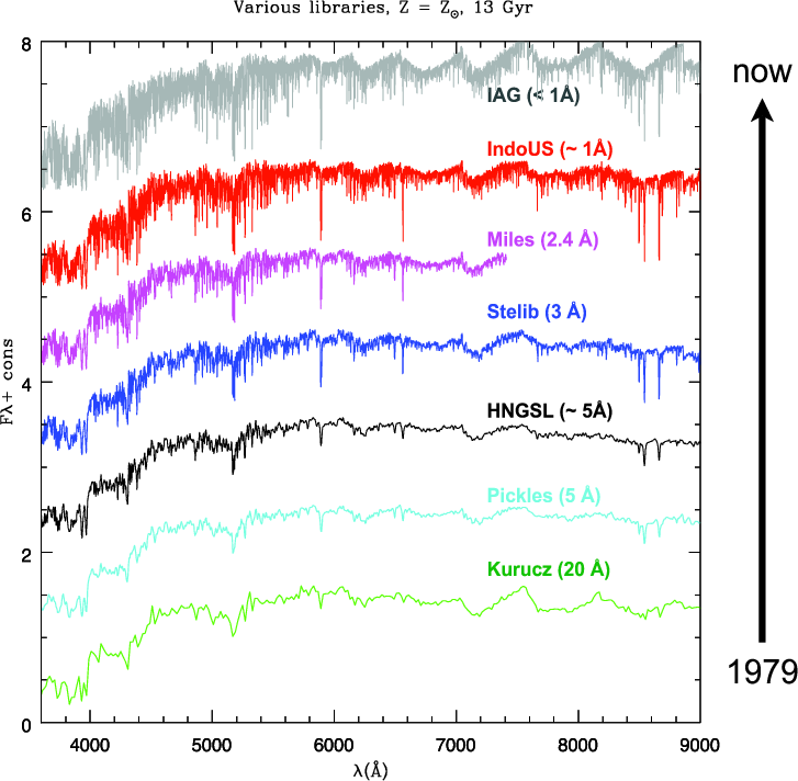
TP-AGB stars are short-lived, cool but luminous components of evolved stellar populations that tend to be more prominent at low metallicities. Due to the short lifetime of this stellar phase, as well as the inherent instability of the pulsations, such stars are difficult to model. Yet due to their relatively high luminosities (see figure 3) they can significantly alter the mass-to-light (M_* /L) ratio of intermediate-age populations and it is thus important to properly include them. Previously, several different theoretical and semi-empirical recipes had been used in stellar population synthesis models leading to large discrepancies between SSP spectra (Vassiliadis and Wood 1993; Maraston 1998). Attention has been focused on these stars since Maraston (2005) raised this issue, leading to rapid progress in the modelling (Marigo and Girardi 2007), largely reducing these differences in the broad-band photometry.

The emission of SSPs near 10 Myr is dominated by luminous red supergiants, showing that more problems exist in the NIR than only TP-AGB stars. At higher spectral resolution in the NIR, comparisons of SSPs based on different libraries of synthetic stellar spectra and different isochrones show large residuals in the whole range from 1 to 2.5 μm and in particular for young to intermediate ages (A. Lançon, talk at workshop). Additionally, ages derived from NIR and optical spectroscopy are discrepant by factors of two in this age regime. Resolving these problems will surely lead to improved predictions of stellar population models at all wavelengths.

EHB stars represent the most luminous hot component in old stellar populations. Understanding these stars and implementing them in SSP codes is important because they could be mistaken for low-level star formation in more evolved, early-type galaxies. Unfortunately, the evolution of EHB stars is not fully understood. While HB morphology may be dependent upon metallicity, some metal-rich stellar populations show HB stars bluer than expected (Heber 2008). The second-parameter problem with the morphology of the horizontal branch (for a review see Catelan 2009) will need to be solved before significant progress can be expected in this field. Meanwhile, the comparison between model SSP spectra and the data at old ages is affected by these uncertainties (Ocvirk 2010).

Blue straggler stars are, as the name suggests, stars that extend beyond the main sequence turn-off. Their origin is still unknown, though it is believed to be associated with binary star evolution, either through mass transfer or merging (Tian et al. 2006; Ferraro et al. 2006). As with EHB stars, blue stragglers can affect the interpretation of early-type spectra giving younger average ages. These stars point towards a fundamental limitation of current SSP modelling, in that effects of binary evolution are not included. While this causes little difference in most cases, in some situations (such as where blue stragglers may dominate) recent binary stellar population models may be more suitable (Han, Podsiadlowski, and Lynas-Gray 2007). In young populations, massive binaries have, however, also been claimed to be generally important (Eldridge and Stanway 2009).

The reader is also referred to the series of papers Conroy, Gunn, and White (2009); Conroy and Gunn (2010b) for a recent systematic study of some of the uncertainties affecting SSP models.

Yet, even with all these remaining issues, SSP modelling has advanced significantly in recent years, with simple Charlot & Bruzual (2010, in preparation) exponentially-declining SFH + burst models able to reproduce 1000’s of optical SDSS spectra (of ~ 5Å resolution) to a few percent (see Section 4.4.4).