![[ ∑ ]2
2n∑ Fi ---Mi=1akSi[tk,Z0,T0]
χ= σi ,
i=0](walcher_ms16x.png)
As has been mentioned in Section 2.1.1, the stellar SED of a galaxy can be represented by a sum over the SEDs of individual SSPs with appropriate weights which reflect the SFH. As long as any complications, such as dust, can be neglected this is a linear problem, i.e. a matrix inversion. More generally, inversion is the attempt to invert the observed galaxy SED onto a basis of independent components (SSPs, dust components) drawn from a SED model. Inversion is typically used for spectral data and a big success of modern stellar population models and inversion codes is that we can now fit the models to data to better than 5% in the optical wavelength range (see Section 4.4.4).
Nearly all inversion methods start with assumptions that reduce the complex physics of SEDs (see Eq 1) to a problem that can be written as a linear function of its parameters. Such assumptions are typically that one deals with a stellar system in which all generations of stars have the same metallicity, i.e. ζ(t) = Z0 and the same attenuation, i.e. T(t) = T0. The problem of solving for the star formation history of a stellar system is then equivalent to defining and minimizing the merit function
|
| (3) |
over all non-negative ak. Here Fi is the observed spectrum in each of n wavelength bins i, σi is the standard deviation and ak are weights attributed to each of M SSP models Si [tk , Z] of age tk and metallicity Z. This merit function is linear in the ak and can thus be solved by standard mathematical methods involving singular value decomposition (e.g. non-negative least squares, bounded least squares)3. A particular advantage of the inversion method is that, besides the assumptions necessary to linearize the problem, no parametrization of the solution is necessary, in particular not of the star formation history. Codes that have been used for scientific analysis are now common and include MOPED (Heavens, Jimenez, and Lahav 2000), PLATEFIT (Tremonti et al. 2004), PPXF (Cappellari and Emsellem 2004), VESPA (Tojeiro et al. 2007), STECKMAP (Ocvirk et al. 2006), STARLIGHT (Cid Fernandes et al. 2005), sedfit (Walcher et al. 2006), NBURSTS (Chilingarian et al. 2007), ULySS (Koleva et al. 2009). Different codes give very comparable results (e.g. Koleva et al. 2008).
There is one problem that has to be addressed when assessing the unparameterized information content of galaxy spectra. All methods relying on singular value decomposition and derived algorithms inherit one of the features, which is that the method tends to search for the smallest number of templates it can use to fit the data. For galaxies, which presumably have a smooth SFH, this feature is a grave caveat concerning the significance of the recovered weights of each population. In particular, the recovery of realistic error bars from a simple bootstrap algorithm is not possible, as the method will tend to always choose some templates over others, inside a range of random errors. One way to address this issue is regularization, detailed in Cappellari and Emsellem (2004, the PPXF program) and Ocvirk et al. (2006, the STECKMAP program).
Another robust exploration of this issue is provided in the code VESPA (described in detail in Tojeiro et al. 2007). As independent parameters (see 4.1) Tojeiro et al. chose 2 values of metallicity and a logarithmic binning in age that can be varied between coarse (3 age bins) and fine (16 age bins). Dust attenuation and varying metallicity are explored by repeating the fit with VESPA over a grid of parameters. Error bars are derived by creating noised representations of the input spectra and repeating the fit n times. The codes main feature in the present context is that it explores the SFHs in an iterative process that goes from coarse to fine resolution. It uses the method described in Ocvirk et al. (2006) to estimate at each step, how many parameters can be recovered for a linear problem perturbed by noise. The best fit will thus only use as many independent stellar populations as required by the data. Nevertheless, one caveat remains, which is that the SFH inside each bin is fixed to be either a constant SFR or such that the light contribution of each age is more or less constant. When recovering parameters such as M/L and in those cases where the age bins are coarse, this will lead to an underestimate of the true uncertainty in this parameter, as compared to a truly non-parametric method.
The main lesson learned from this careful analysis is that from spectra typical of the SDSS (S/N≈20, optical wavelength range), one can recover between 2 and 4 stellar populations described by an age and a metallicity. These values can be improved by a factor of 2 when going either from S/N=20 to S/N=50 or when enlarging the wavelength range to include not only the optical, but also the UV range. Such data will be available in the near future from the XSHOOTER instrument at the VLT. It should be kept in mind, however, that while the formal constraints may be better, the accuracy of the results will then depend critically on the data calibration and model accuracy over a very large wavelength range.
For the optical wavelength range, an exception to the pre-condition of linearity exists in the form of the code STARLIGHT (Cid Fernandes et al. 2005), which is based on simulated annealing and thus does not need linearity. Consistency between STARLIGHT and other codes based on linearity assumptions has been found. Another code avoiding linearity conditions was presented in Richards et al. (2009).
For decomposing MIR spectra into their stellar, PAH, dust continuum, and line emission constituents, Levenberg-Marquardt algorithms have been used (Smith et al. 2007; Marshall et al. 2007, see Section 6.2.2). This allows among other things to compute uncertainties on the derived parameters. With the improvement of dust emission models and in particular the more widespread availability of spectral data, more development in the technicalities of fitting dust spectra can be expected.
Finally, a possible extension of the inversion onto SSP models has been presented in Nolan et al. (2006) and would merit further exploration. Also Dye (2008) has presented a new method, which integrates inversion into a Bayesian framework and applies it to photometric data.
Dust attenuation is important in the optical and UV wavelength ranges. In the context of inversion, the importance of dust is most easily assessed by an iteration over a grid of attenuation values. More sophisticated schemes proceed in an iterative way, i.e. alternate linear inversion and a non-linear minimization scheme (Koleva et al. 2009), or use non-linear minimization schemes for all parameters (Cid Fernandes et al. 2005). Any estimate of the dust attenuation at optical wavelengths from the SED alone (i.e. using neither Balmer decrement, nor UV photometry, nor dust emission) is bound to be uncertain, in particular because no inversion code at present uses a physical model for different attenuations likely experienced by young and old stars.
A very useful way is therefore to normalize the continuum of the observed and model spectra before the fit (e.g. Wolf et al. 2007; Walcher et al. 2009) or even simultaneously with the fit (Koleva et al. 2009). While this takes out any information related to the attenuation, it also allows the freedom from any uncertainties related to continuum calibration and can be thought of as fitting the equivalent widths of the absorption features only. An often under-appreciated caveat is, however, that this procedure throws away some information. In particular (nearly) featureless continua (such as from very young stars) become undetectable, yet still affect the equivalent widths. This “featureless” continuum has to be appreciated in relation to the noise in the observations and, in an intermediate age spectrum can even include a significant contribution of old stars. One expression of this caveat is described in Section 4.6 as the bias occurring when fitting single SSP models to extended SFHs.
Also the effects of forward scattering on the optical SED are not included in Equation 1 and cannot be linearized usefully. In principle the scattering can be modelled through radiation transfer modelling and could thus be included in non-linear minimization schemes. However, radiation transfer modelling is too time-consuming to make this a practical possibility.
In an unpublished contribution to the workshop, Jarle Brinchmann (and collaborators) showed that the 106 spectra of galaxies in the Sloan Digital Sky Survey (SDSS) offer a rich set of tests of the current models and techniques for fitting SEDs in the optical region. For the first series of tests they use a set of 274613 galaxies from the SDSS DR7 with reliable determinations of the emission line fluxes. They fit them using the latest version of the Bruzual and Charlot (2003) models (termed here CB08). In the optical the main improvement in these models is the switch from the Stelib library to the MILES library. The fitting procedure involves classical inversion using a non-negative least squares routine. Additionally they allow for ~ 150 Å wide mismatches between models and spectrum using a smooth final correction. This is necessary because of uncertainties in the spectrophotometry of the data and the models. The result of the NNLS routine is, among others, the mean χ2 of the spectrum, which can in turn be plotted into the classic Baldwin, Phillips, and Terlevich (1981, BPT) diagram [NII]λ6584Å/Hα versus [OIII]λ5007Å/Hβ, shown in Figure 11. Generally, the fit is good, with a reduced χ2 around 1 ± 0.1. Regions can be identified, where the fit is, while still in this range, somewhat worse. These are (A) galaxies with high star formation activity, high excitation and low metallicity, (B) strong, high excitation AGN, and (C) galaxies with high surface mass density (i.e. high mass) and weak emission lines.
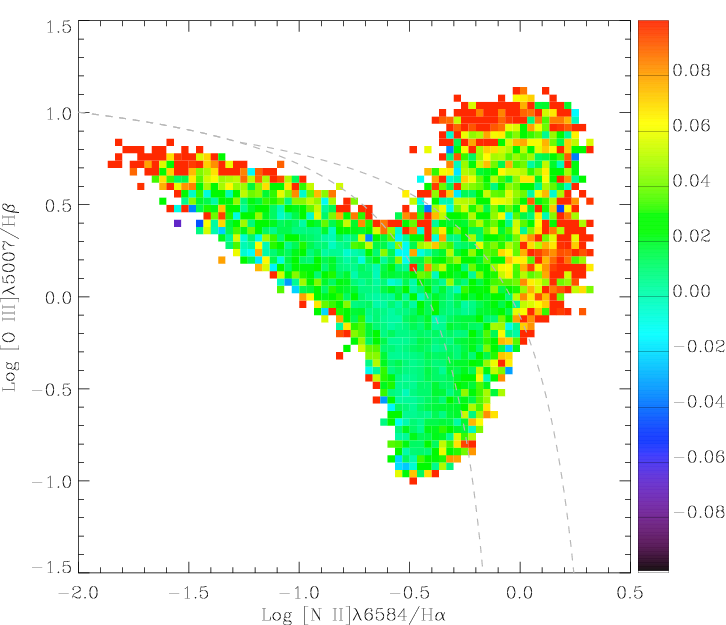
For cases (A) and (B), i.e., the low metallicity starbursts and the high-ionization AGN, they relate the main increase in χ2 to the imperfect masking of some emission lines and to the lack of nebular or AGN continua in the spectra. In addition the BC03 models have some problems with hot stars (e.g. Wild et al. 2007) - the preliminary version CB08 appears to work better, due to a better coverage of hot stars in the spectral library (G. Bruzual, priv. comm.).
For case (C) one of the largest mismatches in the optical is located, as expected, around the Mg features at 5100 Å. This is the region where the enhancement of the abundances of the α elements is known to play an important role. α-enhancement is not covered by the CB08 models. Nevertheless, in the optical the mismatch due to stellar populations is modest, of the order of 0.02 magnitudes.
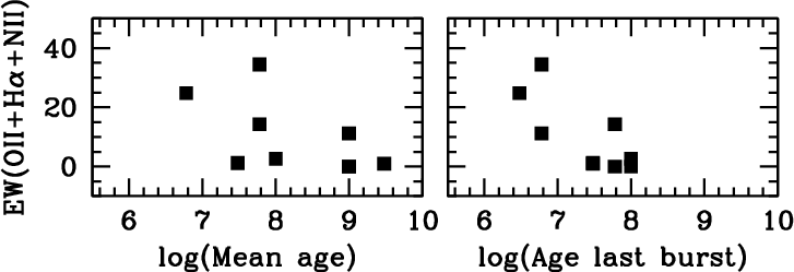
The best method to validate a fitting procedure is to compare the result to independent measurements of the same physical property. This can be done for redshifts, as discussed in section 5, but also for the spectra of nuclear clusters, as done by Walcher et al. (2006) for nine nuclear clusters. The nuclear clusters have multi-aged stellar populations and are as such similar to entire galaxies, and their total stellar masses can be determined dynamically, independent from fitting the stellar spectra.. As shown in Walcher et al. (2006), the stellar M/L ratios from inversion agree with those determined from independent dynamical modelling, albeit with a large scatter. This scatter reflects the general difficulty of constraining the oldest stellar population from SED fitting. Additionally, Walcher et al. (2006) also found that the age of the youngest population as determined from the spectral fitting is correlated to the measured emission line equivalent width, as shown in figure 12 (right). On the other hand, the mean mass-weighted age is not correlated, which is evidence that the fit result is not heavily biased towards the youngest population (in contrast to results from fitting single SSPs, see section 2.1.2).
Another careful work on validation of the spectral fitting procedures was the work by Koleva et al. (2008), who looked at Galactic clusters which had individual stellar spectra and full colour-magnitude diagrams to compare with the results of the fits to the integrated spectra (also compare this with section 2.1.2 for the validation of the predictions of SSP models for integrated spectra).