We refer here in particular to using the “Bayesian fitting” method, in which multi-wavelength SEDs are fit by first pre-computing a discrete set or library of model SEDs with varying degrees of complexity and afterwards determining the model SED and/or model parameters that best fit the data. This approach is favoured in particular for multi-wavelength data, as the problem of solving for the physical parameters is not linear if effects such as dust attenuation, line emission, and dust emission have to be taken into account. In addition, the influence of geometry and the physical conditions of the dust generally make the number of parameters very large, and with many possible degeneracies, thus making non-linear minimization schemes usually impractical.
It is important to realise that the simple fact of pre-computing a set of galaxy models and afterwards determining the one with the lowest χ2 is by itself a Bayesian approach. By choosing which models to compute one introduces a prior, which, while possibly flat in terms of a given parameter, assumes that the data can be represented by that model and that parameter space. By using χ2 as a maximum likelihood estimator one finds the most probable model, or in bayesian terms, the probability of the data given that model. A mathematically much more rigorous description of the method is given in Appendix A of Kauffmann et al. (2003a) and currently builds the basis for Bayesian inference in SED fitting. A more practically oriented description can be found in e.g. section 4 of Salim et al. (2007). In a nutshell, the method uses the fact that — assuming Gaussian uncertainties — the probability of the data (D) given the model (M) is given by P(D|M) ∝ e-χ2∕2 . The prior probability distribution of the model parameters is often taken to be flat within a given parameter range (or flat in log space for larger parameter ranges). To determine the parameters for a specific galaxy dataset, the probabilities for all models are computed and then integrated over all parameters (model space) except the one to be derived, which yields a Probability Distribution Function (PDF). The median and width of this distribution yield the parameter estimate and associated uncertainties. The integration can be repeated and the PDF can be built for all parameters of the models as well as the observables themselves, e.g. with the aim to plot the model and observed fluxes in a fitted band for comparison purposes.
An important step in Bayesian inference for SED fitting is the construction of the library and the prior assumptions (Section 4.5.2). It is equally important to synthesize the correct observables from the models, taking into account response functions and redshifts (Section 3.1).
Bayesian inference for SED fitting has several advantages that minimize potential sources of uncertainties: i) all available measurements contribute to the fit result, ii) the K-correction is integrated, iii) non-linear effects such as from dust are accounted for as part of the models (see section 2.2.2), and thus in a self-consistent way, and finally iv) uncertainties on the derived parameters include measurement uncertainties as well as intrinsic degeneracies. The big caveats concerning this method are the sensitivity to the prior distribution of parameters (the “library”) and, connected to this, the dependence on realistic input physics in the modelling.
The computation of the library is one of the essential steps when using Bayesian inference. It encodes our prior knowledge about the galaxies in the sample, but also our assumptions about which of the physical effects we can safely neglect. Concerning photometric SEDs, a prominent case of neglection is the internal chemical evolution of the model galaxies. This is justified because even the overall metallicity is not measurable from broad-band photometry alone (e.g. Walcher et al. 2008). Also the effects of forward scattering on the optical SED are often not included for computational reasons, but could potentially be important, in particular for starbursts (Jonsson 2006).
One assumption that is generally used is that SFRs tend to decrease monotonically with cosmic time in a given object (with the exception of star formation bursts). This assumption is particularly appropriate for early-type galaxies, which has led to the wide-spread use of so-called τ-models, i.e. exponentially falling functions representing the SFH. However, it is not to be expected that galaxies in reality follow the falling exponential model. The SFHs of dwarf galaxies are expected to be dominated by intermittent bursts (see e.g. Gerola, Seiden, and Schulman 1980). But even for large galaxies, the SFH is not expected to be as smooth as suggested by the simple τ-models. Both semi-analytic (Quillen and Bland-Hawthorn 2008) and hydrodynamic modelling suggest some stochasticity, as discussed in section 4.1. However, due to the smooth variation of SED properties with age and due to the ensuing degeneracies, the τ-models provide reasonable fits to observed SEDs and cannot be easily refuted. Also, they provide a convenient, simple parametrization of SFHs which explains their widespread use.
The danger of using only τ-models lies in the neglect of degeneracies. Let us assume, the χ2 of a specific τ-model is the same as that of a different model, which is the superposition of a smooth SFH and a burst. Both models will have different mean ages and M/L ratios. If they are both included in the library, they will thus lead to a larger error bar. However, if the burst model is omitted, two situations are possible: 1) If we indeed know that strong secondary bursts are unlikely (as e.g. for a sample of morphologically selected early-type galaxies) one will obtain a better estimate of the actual error bar through use of a better prior. 2) If on the other hand one is fitting the entire population of galaxies in a given volume, it is unlikely that no galaxy shows a secondary burst and one will thus — sometimes severely — underestimate the true uncertainty of the recovered parameters. Often “new”, supposedly more precise estimates of galaxy parameters are published that are based on too restrictive priors. In the following we showcase two examples of how to construct a library of star formation histories.
A library for Gaia One of the first cases where Bayesian inference is applied to spectra will be presented in Tsalmantza, et al., (in prep). This is also a good example of how to create a library with a suitable prior for a specific application. The Gaia mission will produce spectra of 106 galaxies at low resolution of R between 50 and 200. Automatic classification of a large number of low-resolution spectra is therefore crucial. Classification is done by comparison to a custom-created library of model galaxy spectra that simulate the properties of the Gaia spectra. This library is used for training and testing of the classification and parametrization algorithms.
Two libraries have been created: The first library is an entirely synthetic one. The library creation starts from the synthetic spectra of 8 typical galaxies produced by PEGASE.2 (Fioc and Rocca-Volmerange 1999). The SFHs of the library spectra are built from analytic prescriptions for either the dependence of SFR on the gas mass (SFR = Mgas p1 ∕p2, late types) or for the SFH directly (SFR=p2.e-t∕p1 ∕p1, early types) as well as parameters forgas infall and galactic winds. In order to create a smooth grid, the input parameters (i.e. p1,p2, gas infall and galactic winds) were allowed to vary over a range of values(see Tsalmantza et al. 2007, 2009). At this point, while of course guided by prior knowledge of the properties of galaxies, the parameter distribution is chosen nearly ad-hoc.
A second library was created based on spectra from the SDSS (DR5, Adelman-McCarthy and et al. 2007). The SDSS spectra were shifted to z=0 and degraded to the resolution of the PEGASE.2 output spectra. They were then classified by comparison to the pre-existing library of purely synthetic spectra through simple χ2-minimization. Using the best fit model spectrum the SDSS library spectra could be extended to cover the Gaia wavelength range and values for the most significant parameters could be assigned to them. Mainly, however, the results of the χ2 fitting were used to judge how the synthetic library compares to the empirical galaxy population in the SDSS. The distribution of input parameters governing the SFHs obtained from the observed SDSS sample can then be used to determine a suitable prior distribution for the synthetic Gaia library. This application is a good example of a case where the prior can be well established based on other observations.
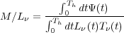
Simplifying M/L determinations A good example of how the appropriate choice of prior can help with constraining the fit is provided by the work of Bell and de Jong (2001, and R. de Jong’s talk at workshop). This work centers on finding the simplest way to derive the mass-to-light ratio of a stellar population. Let us first remember that the stellar mass itself is the product of a galaxies luminosity and its M∕L. M∕L in turn is a function of the star formation history of a galaxy. If the SFR at time t is written as Ψ(t) = dM(t)∕dt and is defined over the entire Hubble time Th, Lν(t) is the luminosity of an SSP at frequency ν, at age t, and with mass dM(t) and Tν(t) is the mean transmission of the ISM at wavelength ν and for the SSP with age t, then we can write
|
| (4) |
This dependence of the M∕L on the SFH means that any prior assumption on the SFH is also a prior assumption on the M∕L.
The crucial simplification inherent in Bell and de Jong (2001) is thus the parametrization of the SFH. This simplification is provided by a prior derived from a hierarchichal formation scenario. Using their scenario, the SFHs of galaxies lead to a situation in which their intrinsic colours show a strong correlation with M/L. The dust attenuation vector is parallel to this relation, and thus the M/L ratio can be derived from a single optical colour with reasonable precision. Nevertheless there is a curvature in the difference between the M/L ratios determined from colours only and M/L ratios determined from an SED fit in the sense that for very blue (young) galaxies and for very old (red) galaxies, the colour-M/L will provide an overestimate, while for intermediate colour, intermediate age galaxies the colour-M/L will be an underestimate.
De Jong & Bell (talk at workshop) explore different possible effects. When comparing a smooth SFH with a single burst, the M/L values have large systematic offsets, due to the lack of faint, old stellar populations in the single burst model. Two burst models do not solve the problem, in particular if the fit is dominated by two young populations. In this case the two-burst model is still not complex enough, it again misses the faint, old population, which is crucial for the mass budget. The problem with the SFH template is further clarified by a comparison between M/L ratios as determined in Bell et al. (2003a) and those derived by k-correct (Blanton and Roweis 2007). While the scatter in the difference is relatively small and there is no systematic trend, there is a systematic offset of about 0.15dex. This can traced to the parametrization of the SFH. Indeed, while Bell et al. (2003a) use pure falling exponentials, the SFH assumed in in k-correct peaks 6 Gyr after the beginning of star formation. Thus, while the resulting SED is not affected, the number of low-mass stars is much higher in the Bell et al. (2003a) SFHs. This uncertainty of 0.15 dex is thus inherent to any mass estimate from SED fitting.
In order to validate the method and its intrinsic accuracy, a number of studies have been performed in the last years.What could be termed “internal validation” is the search for degeneracies and systematics in the models and the method itself (see e.g. Walcher et al. 2008; Wuyts et al. 2009; Longhetti and Saracco 2009).
Extensive testing of stellar mass determinations through SED fitting was done with the COSMOS dataset (Ilbert et al. 2010). SEDs were generated with the stellar population synthesis package of Bruzual and Charlot (2003) assuming a Chabrier (2003) initial mass function (IMF) and an exponentially declining star formation history with a timescale, τ*, ranging from 0.1 to 30 Gyr. The SEDs were generated on a grid of 51 timesteps between 0.1 and 13.5 Gyr. Dust attenuation was simulated using the Calzetti et al. (2000) law with E(B - V ) in the range 0 to 0.5, with steps of 0.1. The colors predicted by this library of SEDs in the COSMOS dataset for the photometric redshift of the galaxy were compared to the observed ones to select the best-fitting templates.
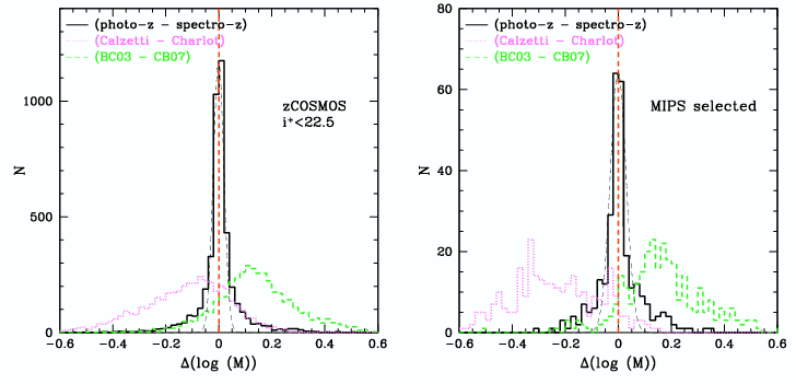
How the potential inaccuracy of the photometric redshifts affects the stellar mass derivations was investigated, and results are displayed in Figure 13. Two spectroscopic samples were used: the zCOSMOS bright spectroscopic sample (Lilly et al. 2007) selected with a magnitude cut only at iAB+ < 22.5 and a spectroscopic follow-up of 24 μm sources selected from S-COSMOS (Sanders et al. 2007). These sources are typically dusty starbursts with 18 < iAB+ < 25. A median difference smaller than 0.002 dex is found between the photo-z and the spectro-z stellar masses, for both spectroscopic samples.
It is interesting to note that the stellar synthesis models have the same effect for both selections, as shown in Figure 13. This is not the case when studying the impact of the attenuation law. The MIPS selection consisting preferentially of dusty galaxies, the difference due to the choice of attenuation (the Calzetti et al. 2000 law in a case, the Charlot and Fall 2000 in the other) is amplified for this sample. The median difference in stellar masses is -0.1 dex for the optical selection and -0.24 dex for the infrared selection.
The impact of the choice of stellar synthesis model on the stellar masses determinations was also examined. Figure 13 presents the difference between stellar masses computed using the Bruzual and Charlot (2003) models and the new models of Charlot and Bruzual (2007, private communication) including a better treatment of the pulsing asymptotic giant branch. A median difference of 0.13–0.16 dex and a dispersion of 0.09 dex is observed. Pozzetti et al. (2007) found a similar difference (0.14 dex) when comparing Bruzual and Charlot (2003) and Maraston (2005) models. Walcher et al. (2008) show that this offset changes with the measured sSFR of the galaxy, in the sense that the masses determined using BC03 for objects with an intermediate sSFR (-12 < log (sSFR) < -9) are, in the mean, more massive by 50% than those determined using CB07. These are the objects where the TP-AGB stars are most likely to contribute significantly to the light in the NIR bands. Objects with lower or higher sSFRs do not show this offset in Walcher et al. (2008).
Ilbert et al. (2010) concluded from this study that the use of photometric redshifts is only a weak source of uncertainty when deriving stellar masses for a sample of galaxies. The uncertainties are dominated by the uncertainties in the SED modeling itself, thus one has to be very cautious about the interpretations when selecting samples where a specific type of model is preferred.
External validation of the method is possible for one parameter in particular, namely the SFR. Using the entire SED to derive the SFR was considered less precise than other methods (based on specific tracers) in Kennicutt (1998). The availability of large samples with UV, optical and NIR photometry have lead to a reappraisal of the method in the last years. Salim et al. (2007) show a detailed comparison based on the data from the SDSS and the Galex satellite. They derive SFRs using the multi-wavelength SED. They then compare these to the SFRs derived by Brinchmann et al. (2004), which used all emission lines that can be usefully measured in the SDSS spectra and detailed modelling of the emission line spectrum to derive dust-corrected, emission-line based SFRs. As shown in their figure 6, the SED-derived SFRs show in general a satisfying agreement. A similar test was performed in Walcher et al. (2008) on a VVDS-SWIRE-GALEX-CFHTLS sample, where the SED SFR was compared to SFRs derived from the [OII]λ3727Å emission line. While the latter are much less accurate than the emission line SFRs from Brinchmann et al. (2004), the agreement between SED and emission line SFR was shown to be satisfying out to a redshift around one (their figure 8). An advantage of obtaining SFRs from broad-band SEDs compared to emission-lines is the time needed to obtain sufficient S/N in the spectra to get the lines. Nevertheless, an interesting residual correlation of SFR difference with stellar mass is found in SED fitting, which remains yet to be fully understood. Another interesting problem exists in early-type galaxies, in which no Hα emission can be measured, yet UV emission is commonly found (see e.g. Salim et al. 2007, Figure 3). This probably is the cause why some objects with no measurable emission lines have relatively high SED SFRs.
In order to test the SFR determinations from SED
fitting at z~1, Salim et al. (2009) extended previous work
to include the mid-IR dust emission. The consensus is that
the mid-IR emission is heated by the UV, and hence traces
the emission of young stars ( 100 Myr) and it therefore
provides a good means to measure the SFR. Deep MIPS 24
μm imaging exists for the Extended Groth Strip (EGS), as
well as redshifts assembled in the context of the DEEP2
survey. The rest-frame 12 μm emission was converted to a
total dust luminosity using the Dale and Helou (2002)
prescriptions. Using the dust attenuation determined
from fitting the UV-optical SED one can calculate the
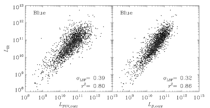
dust-corrected UV and B-band luminosities. These
correlate well with the 24μm luminosity as seen in figure
14. Turning the IR luminosity into a SFR using the
relations of Kennicutt (1998), the best correlation was
found for an SED-SFR measured over the last 1–3
Gyr. That the mid-IR may be heated by older stars
recently received support in a study by Kelson and
Holden (2010), which predicts that C-type TP-AGB stars
(~1.5 Gyr old) can produce a large fraction of the mid-IR
flux.
100 Myr) and it therefore
provides a good means to measure the SFR. Deep MIPS 24
μm imaging exists for the Extended Groth Strip (EGS), as
well as redshifts assembled in the context of the DEEP2
survey. The rest-frame 12 μm emission was converted to a
total dust luminosity using the Dale and Helou (2002)
prescriptions. Using the dust attenuation determined
from fitting the UV-optical SED one can calculate the
dust-corrected UV and B-band luminosities. These
correlate well with the 24μm luminosity as seen in figure
14. Turning the IR luminosity into a SFR using the
relations of Kennicutt (1998), the best correlation was
found for an SED-SFR measured over the last 1–3
Gyr. That the mid-IR may be heated by older stars
recently received support in a study by Kelson and
Holden (2010), which predicts that C-type TP-AGB stars
(~1.5 Gyr old) can produce a large fraction of the mid-IR
flux.
Nevertheless, for some very red objects in their sample, some SED SFRs seriously underpredict the SFR determined from the IR emission. These galaxies have a dominant old population, where the IR may have little to do with SF. Indeed, for the case of early-type galaxies Johnson et al. (in prep.) find that it is important to consider the fraction of the stellar emission absorbed redwards of 4000 Å in order to obtain a good prediction for the measured FIR emission. Neglecting this emission leads to an underprediction of the FIR emission by factors of up to 5.
Stellar mass is the second parameter that can in principle be calibrated empirically, with the hope of deriving the normalization of the M/L ratio, in other words the choice of IMF. However, uncertainties related to technical questions concerning the SED fitting and the dynamical mass measurements are still too high to derive very accurate overall IMF normalizations (see e.g. Cappellari et al. 2006; Salucci, Yegorova, and Drory 2008). Careful attention should also be paid to issues such as the contribution of dark matter, recycled gas, and other dark components. In the formulation of Bell and de Jong (2001), the slope of the colour-M/L relation is independent of the IMF, but the normalization depends on it. For this reason Bell and de Jong (2001) used the maximum disk approximation to provide an upper boundary of the total mass in stars allowed in spiral galaxies. They thus confirm that the Salpeter IMF leads to too high M/L ratios and they adapt the normalization of the colour-M/L relation to be 0.15 dex below Salpeter. Thus a Kroupa or Chabrier IMF seem to be good choices (see section 2.1.1). Variations between stellar population models and in dependence on the available data range also need to be considered carefully (see e.g. van der Wel et al. 2006). As many more independent mass tracers exist, which require careful assessment, the interested reader is pointed to de Jong & Bell (in prep.) for further discussion of this topic.