5.1 Methods

5.1.1 Empirical techniques

Early on, the first empirical methods proved extremely powerful despite their simplicity (see e.g. Connolly et al. 1995a; Brunner et al. 1997; Wang, Bahcall, and Turner 1998). This was partly due to their construction, which should provide both accurate redshifts and realistic estimations of the redshift uncertainties. Even low-order polynomial and piecewise linear fitting functions do a reasonable job when tuned to reproduce the redshifts of galaxies (see e.g. Connolly et al. 1995a). These early methods provided superior redshift estimates in comparison to template-fitting for a number of reasons. By design the training sets are real galaxies, and thus suffer no uncertainties of having accurate templates. Similarly as the galaxies are a subsample of the survey, the method intrinsically includes the effects of the filter bandpasses and flux calibrations

One of the main drawbacks of this method is that the redshift estimation is only accurate when the objects in the training set have the same observables as the sources in question. Thus this method becomes much more uncertain when used for objects at fainter magnitudes than the training set, as this may extrapolate the empirical calibrations in redshift or other properties. This also means that, in practice, every time a new catalogue is created, a corresponding training set needs to be compiled.

The other, connected, limitation is that the training set must be large enough that the necessary space in colours, magnitudes, galaxy types and redshifts is well covered. This is so that the calibrations and corresponding uncertainties are well known and only limited extrapolations beyond the observed locus in colour-magnitude space are necessary.

The simplest and earliest estimators were linear and polynomial fitting, where simple fits of the empirical training set in terms of colours and magnitudes with redshift were obtained (see e.g. Connolly et al. 1995a). These could then be matched to the full sample, giving directly the redshifts and their uncertainties for the galaxies. Since then further, more computational intensive algorithms, have been used, such as oblique decision tree classification, random forests, support vector machines, neural networks, Gaussian process regression, kernel regression and even many heuristic homebrew algorithms.

These algorithms all work on the idea of using the empirical training set to build up a full relationship between magnitudes and/or colours and the redshift. As each individual parameter (say the B -V colour) will have some spread with redshift, these give distributions or probabilistic values for the redshift, narrowed with each additional parameter. This process, in terms of artificial neural networks, is nicely described by Collister and Lahav (2004), who use this method in their publicly available photo-z code ANNz (described in the same paper). They also discuss the limitations and uncertainties that arise from this methodology.

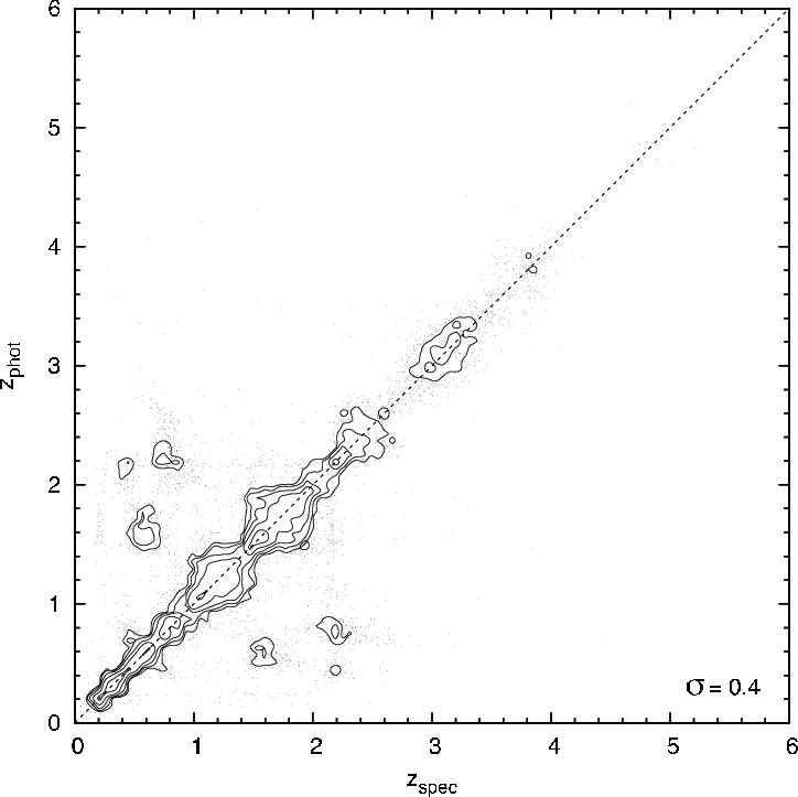
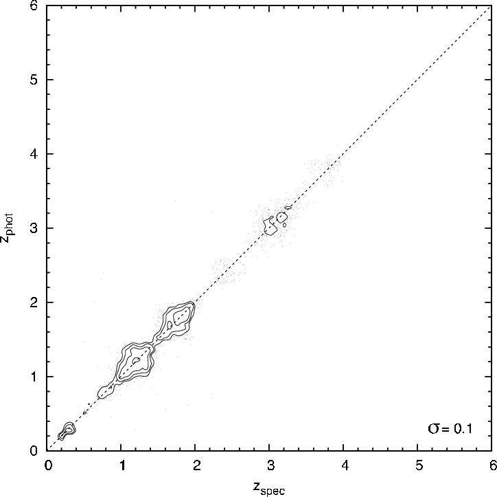
Machine learning algorithms (of which neural networks is one) are one of the strengths of the empirical method. These methods are able to determine the magnitude/colour and redshift correlations to a surprising degree, can handle the increasingly large training sets (i.e. SDSS) and return strong probabilistic estimates (i.e. well constrained uncertainties, see figure 16) on the redshifts (see Ball et al. 2008a, for a description of machine learning algorithms available and the strong photo-z constraints possible). In addition, machine learning algorithms are also able to handle the terascale datasets now available for photo-z determination rapidly, limited only by processor speed and algorithm efficiency (Ball, Loveday, and Brunner 2008b).

The additional benefit of the empirical method with machine learning, now increasingly being used, is that the constraining inputs for the photo-zs are not limited to the galaxies SED. Suggested first by Koo (1999), properties such as the the bulge-to-total flux ratio (e.g. Sarajedini et al. 1999), surface brightness (e.g. Kurtz et al. 2007), petrosian radii (e.g. Firth, Lahav, and Somerville 2003), and concentration index(e.g. Collister and Lahav 2004) have all been used in association with the magnitudes and colours to constrain the redshift, some codes even bringing many of these together (e.g. Wray and Gunn 2008).

5.1.2 Template Fitting

Unlike the empirical method, the template-based method is actually a form of SED fitting in the sense of this review (see e.g. Koo 1985; Lanzetta, Yahil, and Fernández-Soto 1996; Gwyn and Hartwick 1996; Pello et al. 1996; Sawicki, Lin, and Yee 1997). Put simply, this method involves building a library of observed (Coleman, Wu, and Weedman 1980, is a commonly used set) and/or model templates (such as Bruzual and Charlot 2003) for many redshifts, and matching these to the observed SEDs to estimate the redshift. As the templates are “full” SEDs or spectra, extrapolation with the template fitting method is trivial, if potentially incorrect. Thus template models are preferred when exploring new regimes in a survey, or with new surveys without a complementary large spectroscopic calibration set. A major additional benefit of the template method, especially with the theoretical templates, is that obtaining additional information, besides the redshift, on the physical properties of the objects is a built-in part of the process (as discussed in section 4.1). Note though, that even purely empirical methods can predict some of these properties if a suitable training set is available (see e.g. Ball et al. 2004).

However, like empirical methods, template fitting suffers from several problems, the most important being mismatches between the templates and the galaxies of the survey. As discussed in section 2, model templates, while good, are not 100% accurate, and these template-galaxy colour mismatches can cause systematic errors in the redshift estimation. The model SEDs are also affected by modifiers that are not directly connected with the templates such as the contribution of emission lines, reddening due to dust, and also AGN, which require adapted templates (see e.g. Polletta et al. 2007; Assef et al. 2010).

It is also important to make sure that the template set is complete, i.e. that the templates used represent all, or at least the majority, of the galaxies found in the survey (compare also Section 4.5.2). This is especially true when using empirical templates, as these are generally limited in number. Empirical templates are also often derived from local objects and may thus be intrinsically different from distant galaxies, which may be at different evolutionary stage. A large template set is also important to gauge problems with degeneracies, i.e. where the template library can give two different redshifts for the same input colours. Another potential disadvantage of template fitting methods comes from their sensitivity to many other measurements to about the percent level, e.g., the bandpass profiles and photometric calibrations of the survey.

For implementations of the template fitting, the method of maximum likelihood is predominant. This usually involves the comparison of the observed magnitudes with the magnitudes derived from the templates at different redshifts, finding the match that minimizes the χ² (compare section 4.5). What is returned is the best-fitting (minimum χ²) redshift and template (or template+modifiers like dust attenuation). By itself this method does not give uncertainties in redshift, returning only the best fit. For estimations of the uncertainties in redshift, a typical process is to propagate through the photometric uncertainties, to determine what is the range of redshifts possible within these uncertainties. A good description of the template-fitting, maximum likelihood method can be found in the description of the publicly available photo-z code, hyperz in Bolzonella, Miralles, and Pelló (2000).

As mentioned above, one of the issues of the templates is the possibility of template incompleteness, i.e.  not having enough templates to describe the galaxies in the sample. Having too many galaxies in the template library on the other hand can lead to colour-redshift degeneracies. One way to overcome these issues is through Bayesian inference: the inclusion of our prior knowledge (see Section 4.5), such as the evolution of the upper age limit with redshift, or the expected shape of the redshift distributions, or the expected evolution of the galaxy type fractions. As described in Section 4.5, this has the added benefit of returning a probability distribution function, and hence an estimate of the uncertainties and degeneracies. In some respects, by expecting the template library to fit all observed galaxies in a survey, the template method itself is already Bayesian. Such methods are used in the BPZ code of Benítez (2000), who describes in this work the methodology of Bayesian inference with respect to photo-z, the use of priors and how this method is able to estimate the uncertainty of the resulting redshift.

It should be noted that, while public, prepackaged codes might provide reasonable estimates for certain types of sources, no analyses should proceed without cross-validation and diagnostic plots. There are common problems that appear in data sets and issues that need to be understood first, and worked around, if possible (see e.g. Mandelbaum et al. 2005, for a comparison of some public photo-z codes). Some further public photo-z codes include kphotoz (Blanton et al. 2003), zebra (Feldmann et al. 2006), Le Phare (Arnouts et al. 1999; Ilbert et al. 2006, 2009a) and the code by Assef et al. (2008).