5.2 Calibration and error budgets
Redshift errors are ultimately data-driven: they typically
scale with 1 + z given constant wavelength resolution of
most filter sets; they also scale with photometric error in a
transition regime between ~ 2% and ~ 20%. Smaller errors
are often not exploited due to mismatches between data
and model arising from data calibration and choice of
templates, while large errors translate non-linearly into
weak redshift constraints. If medium-band resolution is
available, QSOs show strong emission lines and lead
to deeper photo-z completeness for QSOs than for
galaxies.
Photometric redshifts have limitations they share with
spectroscopic ones, and some that are unique to them: as
in spectroscopy, catastrophic outliers can result from the
confusion of features, and completeness depends on SED
type and magnitude. Two characteristic photo-z problems
are mean biases in the redshift estimation and large
and/or badly determined scatter in the redshift errors.
Catastrophic outliers result from ambiguities in colour
space: these are either apparent in the model and allow
flagging objects as uncertain, or are not visible in the
model but present in reality, in which case the large error
is inevitable even for unflagged sources. Empirical models
may be too small to show local ambiguities with large
density ratios, and template models may lack some SEDs
present in the real Universe.
Remedies to these issues include adding more
discriminating data, improving the match between data
and models as well as the model priors, and taking care
with measuring the photometry and its errors correctly in
the first place. Photo-z errors in broad-band surveys
appear limited to a redshift resolution near 0.02 × (1 + z),
a result of limited spectral resolution and intrinsic variety
in spectral properties. Tracing features with higher
resolution increases redshift accuracy all the way to actual
spectroscopy. Future work among photo-z developers
will likely focus on two areas: (i) Understanding the
diversity of codes and refining their performance; and (ii)
Describing photo-z issues quantitatively such that
requirements on performance and scientific value can be
translated into requirements for photometric data, for the
properties of the models and for the output of the
codes.
5.2.1 Template accuracy
In general, template-based photo-z estimates depend
sensitively on the set of templates in use. In particular, it
has been found that better photo-z estimates can be
achieved with an empirical set of templates (e.g. Coleman,
Wu, and Weedman 1980; Kinney et al. 1996) rather
than using stellar population synthesis models (SPSs;
e.g. Bruzual and Charlot 2003; Maraston 2005,
see Section 2) directly. Yet the models are what are
commonly used to compute stellar masses of galaxies.
Since the use of these templates do not result in very good
photometric redshifts, what is usually done, is to first
derive photometric redshifts through empirical templates,
and then estimate the stellar masses with the SSP
templates. Obviously this is not self-consistent.
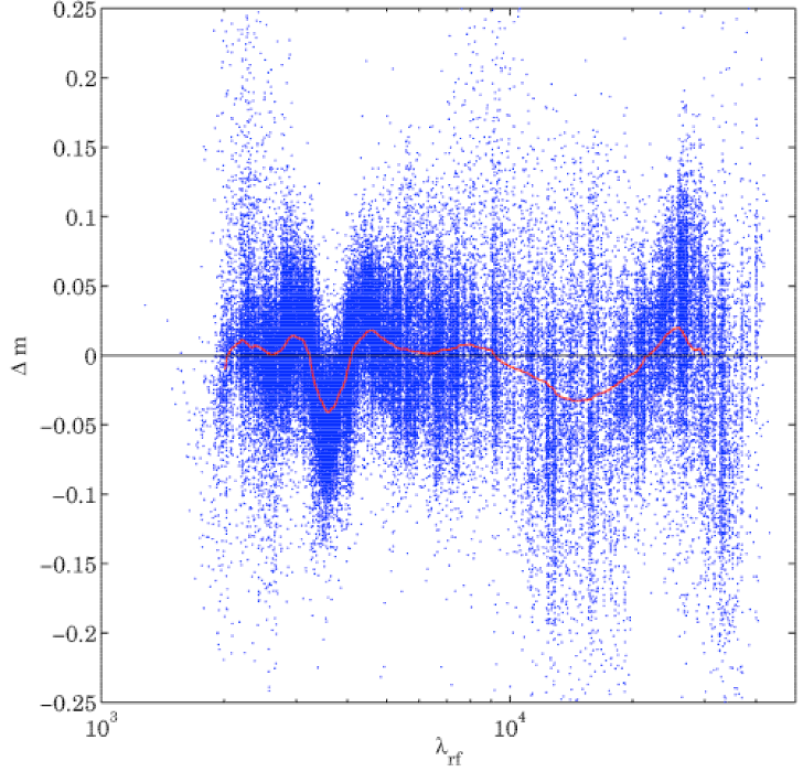
To investigate what causes the poorer photo-z estimates
of synthetic templates, Oesch et al. (in prep.) used the
photometric data in 11 bands of the COSMOS survey
(Scoville et al. 2007), together with redshifts of the
zCOSMOS follow-up (Lilly et al. 2007) and fit the data
with SSP templates. In the resulting rest-frame residuals
they identified a remarkable feature around 3500 Å,
where the templates are too faint with respect to the
photometric data, which can be seen in figure 17.
The feature does not seem to be caused by nebular
continuum or line emission, which they subsequently
added to the original SSP templates. Additionally,
all types of galaxies suffer from the same problem,
independent of their star-formation rate, mass, age, or dust
content.
Similar discrepancies have been found previously
by Wild et al. (2007); Walcher et al. (2008), who
found a ~ 0.1 mag offset in the Dn(4000) index. As
this spectral break is one of the main features in the
spectrum of any galaxy, it is likely that the poor photo-z
performance of synthetic templates is caused by this
discrepancy. The cause of the discrepancy has been
identified as a lack of coverage in the synthetic stellar
libraries used for the models. It will thus be remedied in
the next version of GALAXEV (G. Bruzual, priv.
comm.).
5.2.2 Spectroscopic Calibration of Photo-zs
One of the strong benefits of the template method is that
any spectroscopic subsample of a survey can be used to
check the template-determined photo-zs. This can also be
done for the empirical methods, yet for this a very large
spectroscopic sample is necessary such that it can be
divided into a large enough training set and testing
sets.
With the existence of a test spectroscopic sample, it is
then possible to calibrate the template library, leading to acombined empirical-template method. This means to
correct for errors in the photometric calibration or even the
correction of the templates themselves for example to allow
for the evolution of galaxies with a small library, or to
account for inaccurate models (see section 2). Such
calibration is typically an iterative process, in which the
photometry and/or template SEDs are modified to
minimize the dispersion in the resulting photometric
redshifts.
The simplest kind of calibration involves adding small
zero-point offsets to the photometry uniformly across the
sample. This does not imply that the photometry is
incorrectly calibrated (though in practice the absolute
calibration may well have small errors in the zero-point),
but rather that there is often a mismatch between the real
SEDs of galaxies and the templates used to fit them. The
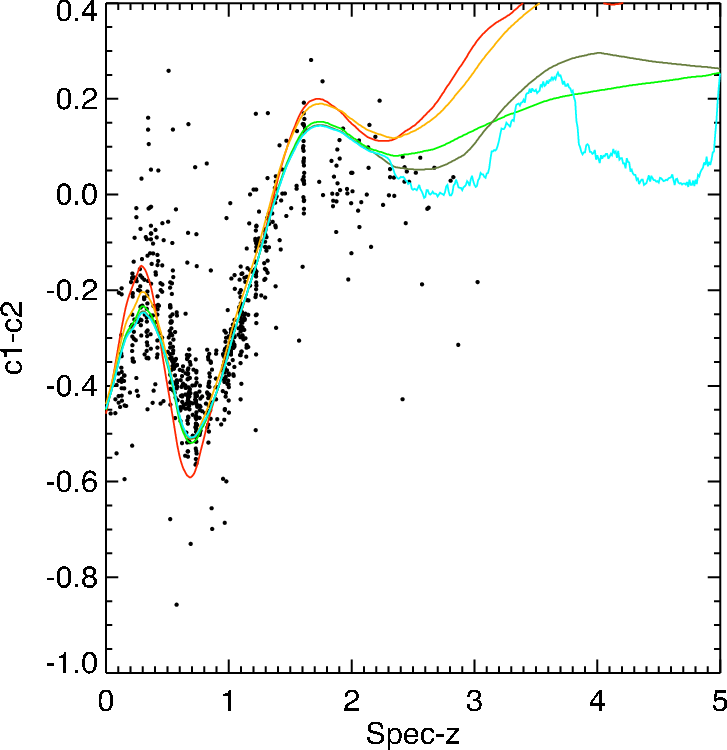
calibration is meant to minimize those differences. Plotting
color-color or color-redshift diagrams (figure 18) with the
template SEDs overlaid will often indicate bulk offsets
between the two.
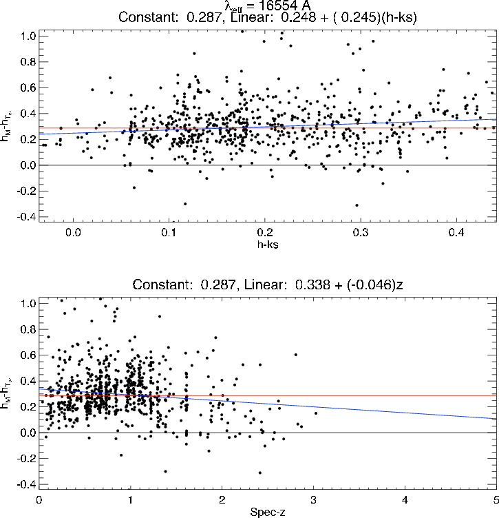
A more instructive approach, however, is to compute
the residuals between the predicted magnitude of the
best-fit template at the spectroscopic redshift and the
observed magnitude (for more details, see Brodwin
et al. 2006a,b). These residuals can be plotted versus color
or redshift for added diagnostic power. In the example in
Figure 19, there appears to be an effective magnitude
offset of ≈ 0.3 mags in the H-band.
Applying such effective zero-point adjustments in all
bands in an iterative process minimizes the mismatch
between the data and the templates, and hence minimizes
the resultant photometric redshift dispersion, as shown in
Fig. 20.
Such calibration phases are used in the works of
Brodwin et al. (2006a) and as “template-optimization” in
the codes zebra (Feldmann et al. 2006) and Le Phare
(Ilbert et al. 2006, 2009a) which use template fitting with
Bayesian inferences and this calibration phase to give the
most accurate photometric redshifts possible with the
template approach.
With the most accurate photometric redshifts possible,
the template-fitting can then be used to estimate physical
properties such as stellar masses, star-formation rates, etc.
(see section 6).
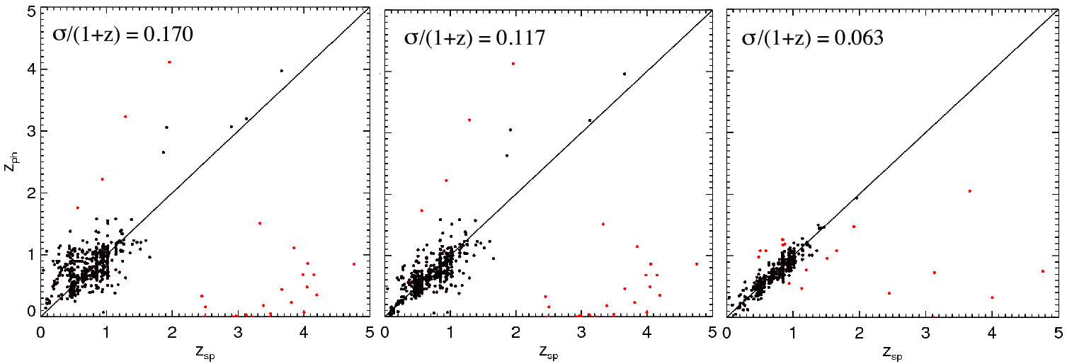
Fig. 20 : Iterative improvement in photometric redshift estimation via this simple calibration technique.
[Courtesy M. Brodwin]
5.2.3 Signal-to-noise Effects
Margoniner and Wittman (2008) have specifically
investigated the impact of photometric signal-to-noise (SN)
on the precision of photometric redshifts in multi-band
imaging surveys. Using simulations of galaxy surveys with
redshift distributions (peaking at z ~ 0.6) that mimics
what is expected for a deep (10-sigma R band = 24.5
magnitudes) imaging survey such as the Deep Lens
Survey (Wittman et al. 2002) they investigate the
effect of degrading the SN on the photometric redshifts
determined by several publicly available codes (ANNz,
BPZ, hyperz)
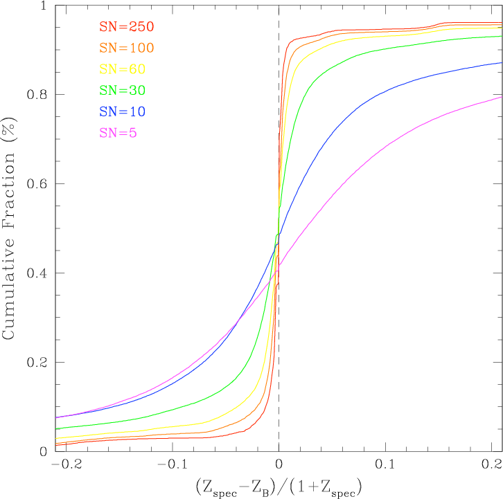
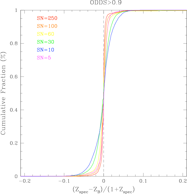
Figure 21 shows the results of one set of their simulations
for which they degraded the initially perfect photometry to
successively lower SN. In these unrealistic simulations all
galaxies have the same SN in all bands. The figure shows
the cumulative fraction of objects with δz smaller than a
given value as a function of δz. The left panel shows the
cumulative fraction for all objects, while the right panel
shows galaxies for which the BPZ photo-z quality
parameter, ODDS > 0.9. The number of galaxies in
the right panel becomes successively smaller than the
number in the left as the signal-to-noise decreases (64%
of SN=250, and only 6.4% of SN=10 objects have
ODDS > 0.9), but the accuracy of photo-zs is clearly
better.
The results of this work show (1) the need to include
realistic photometric errors when forecasting photo-zs
performance; (2) that estimating photo-zs performance
from higher SN spectroscopic objects will lead to overly
optimistic results.